I chose my step response to be 170 as that was a reasonable speed
for what I had done in prior labs and was greater than 50% of the maximum u
which was 255 due to PWM limits. I still used 255 as my PWM when u = 1
since in a prior lab I fixed the straightness of my car and managed to remove
my calibration factor.
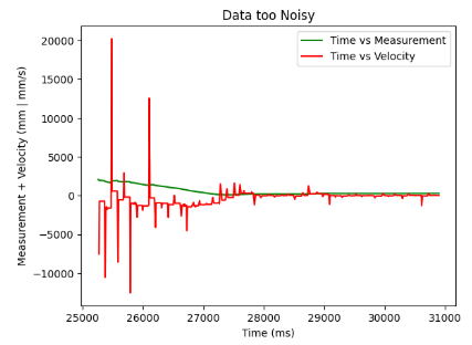
After that I ran the vehicle and collected data. However, due to noise issues
in the velocity data which many other students had as well, I
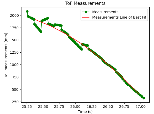
then snipped the data and plotted a line of best fit to my ToF data.
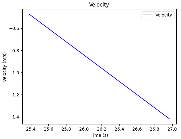
Using this, I then took the derivative of this line to get the velocity.
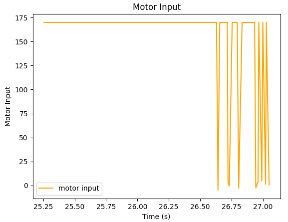
Plots of the noisy data, the true ToF measurements, the line of best fit, its velocity,
as well as the motor input are seen below.
Broken Down: Plot 1 is the ToF measurement raw and the computed velocity
with raw data.
As one can see, there is a lot of high noise in the velocity.
ToF measurements: As one can see I then made my measurement take the line of best fit which
the comparison can be seen in the second plot. Since the line of best fit is just a
2nd degree polynomial, I took its derivative to get the velocity. In the last plot,
one can see the motor input is consistently 170 until around when it is near its target.
.
Given these findings, I saved the data
then found the steady state speed to be 1.42 m/s.
90% of that is 1.278 and therefore, I used the line representing the velocity
to find my rise time to be roughly 1,274 ms by subtracting the
timestamp that was associated with 1.278 and the initial timestamp in the data.
Computing A and B
To get A and B I used the following equations:
A = [[0 1],[0 -d/m]]
B = [[0],[1/m]]
I then computed d as .667 / 1.42 which came out to be .469 kg/s.
I got .667 due to my motor input being 170/255 and 1.42 was my steady state time.
Then to compute m, I computed -d * 1.274 / ln(.1) which was .25949 kg.
Given all of this my matrices were:
A = [[0 1],[0 -1.81]
B = [[0],[3.86]]
Initialize KF
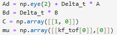
After this I put these matrices as np arrays in python and then compute Ad, Bd, C, and mu
as follows:
My ToF sensors are flipped so doing C as [-1 0] flipped
my KF. As a result, I did [1 0]. To initialize my state vector,
I used the measurements from my saved data and similarly had to keep
the initial mu as positive.
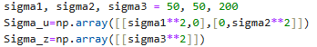
Next, I needed to specify my covariance matrices
depending on the confidence I had for my process versus sensor.
I ended up needing to adjust these values quite a bit from my initial
guesses where I computed them using
sqrt(100/sampling time) for sigma1, sigma2 and sqrt(100/sensor variance).
I got sampling time by averaging the time between each sensor measurement,
and I got sensor variance by computing the variation in measurements when
my robot was stationary.
These computations gave me sigma1, sigma2, sigma3 = 85, 85, 19.
After implementing the simulation,
I found this would trust the sensor measurements too much and therefore,
overfit to the data. To get it to work better, I drastically increased the sigma_z
value compared to the process getting it to be
sigma1, sigma2, sigma3 = 50, 50, 200. This setup of values
also ended up working on the hardware.
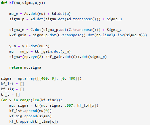
Implement and test your KF in Jupyter
After that to test my parameters and tune them,
I implemented the KF function in Jupyter lab and then ran through
my data using the KF. I scaled my input to .667.
The function and process can be seen below:
As mentioned earlier, my first set of sigma parameters were overfitting to the
ToF measurements. As a result, I decided to increase my trust in my process a lot
more. I also flipped the signs on my initial mu and C matrix, as
they were the opposite of the example code since I get my measurements
differently. A and B as computed earlier along with their derivative equivalents
(where Delta_T was computed using the time between measurements) worked perfectly on their first try,
as well as my initial sigma of [[400, 0],[0 400]].
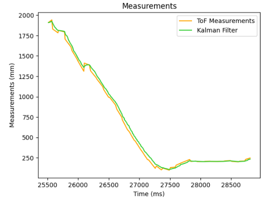
I share three charts below which demonstrate as described.
Chart 1: Final Parameters / Good Filter. Implemented on hardware.
Chart 2: Flipped C and initial mu. These values caused it to be the inverse of
what was desired. This is because mu inverted my initial position estimate and C
inverted the expectation of what the measurements were estimating.
Chart 3: The figure where Sigma1, Sigma2, Sigma3 = 85, 85, 19. I trusted my sensor measurements
too much and overfit. As a result, via trial and error I parameter tuned
the covariance matrices as mentioned above.
Below, I include a list of the parameters that impact performance:
A / B / Ad / Bd = State space matrices used to multiple by mu and u respectively.
Changing these values will impact how control input and prior state estimate
the new state. Ad / Bd take into account the change in time (Delta_T).
C = Used to map expected direction of measurement.
Flipping C from [-1 0] to [1 0] in Chart 2 above resulted in
the KF estimating the measurement positively accurately.
initial mu = The initial state. Using -ToF gave me a negative
initial starting point as seen in Chart 2 above. Flipping it
gave the correct initial estimate.
initial sigma = The initial confidence matrix. A larger matrix
indicates less confidence in location. Too small of a sigma means you
may be more confident in your initial measurement than you should be.
Sigma_u / Sigma_z = Confidence matrices corresponding to
processes and measurement respectively. Their relative values indicate
the degree you trust your process versus your measurements. I increased
sigma_z which resulted in me trusting my process more.
Implement the Kalman Filter on the Robot
C Code
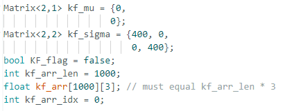
First, I initialized the properly library and
stated using namespace BLA and then declared the global variables
as seen below:
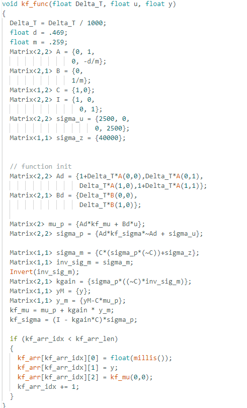
After these global definitions,
I implemented kf_func() which the final form can be seen below.
Some bugs I came across while debugging kf_func was that since
all my computations were in seconds for individual values,
I had to take Delta_T and divide it by 1000 since it was in ms or else it would
cause an integer overflow error and return nan values.
Other bugs also included originally using sigma_mu as kf_mu
in situations where there weren't measured values.
However, in the end this was my kf_func.
After using this as my kf_func, I then needed to call this function.
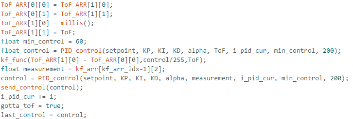
The first case was just standard, use a ToF measurement when you have a ToF
measurement. The code snippet can be seen below. But basically,
I just get the expected control with my PID_control function,
I use that as my u by taking it as a percentage of 255 and for my
y I use my actual ToF measurement.
The other case I need to consider is if there is no new ToF value.
For this case I use the last ToF measurement as my y, the time from that ToF measurement
as my Delta_T, and last_control output as my u.
I run it through my kalman filter to get my measurement
which I use instead of my ToF measurement for the PID_control.
A code snippet is seen below.
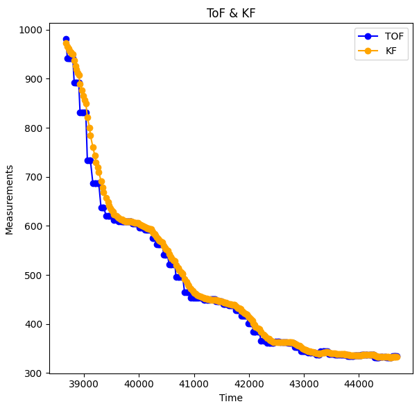
After that, I ran my code on the robot and videod it
and sent the data of the ToF sensors and the Kalman Filter over.
The video is seen below:
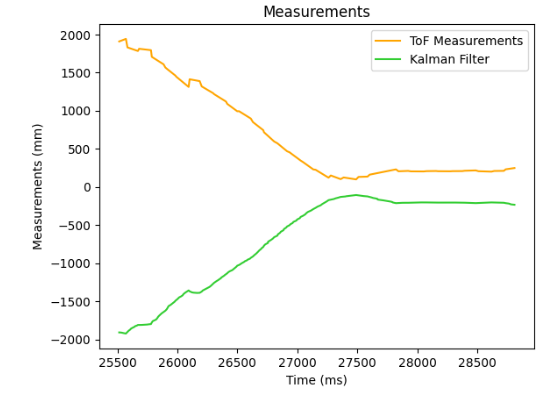
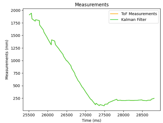
There are two charts I share below.
The first is the whole chart, as one can see the ToF sensor is a little confused
causing the initial jump start. However, it soon figures out the true distance
from the wall and the kalman filter follows it and the performance is as
expected.
The second is just a zoomed in version focusing solely on the relevant part of the graph.
As one can see, the Kalman Filter is estimating its expected position pretty well and
even while the ToF sensor doesn't have a new measurement, the KF does have a good estimate
of its true position.