For this portion of the code, I just repurposed my
PID orientation control code which exists in the function stunt_s2(yaw)
which the documentation for can be referenced in my Lab 8 report. I chose
this one since I have good working orientation control that is easily
usable for this purpose. This allows me to stop it at each measurement
so I can get more accurate measurements.
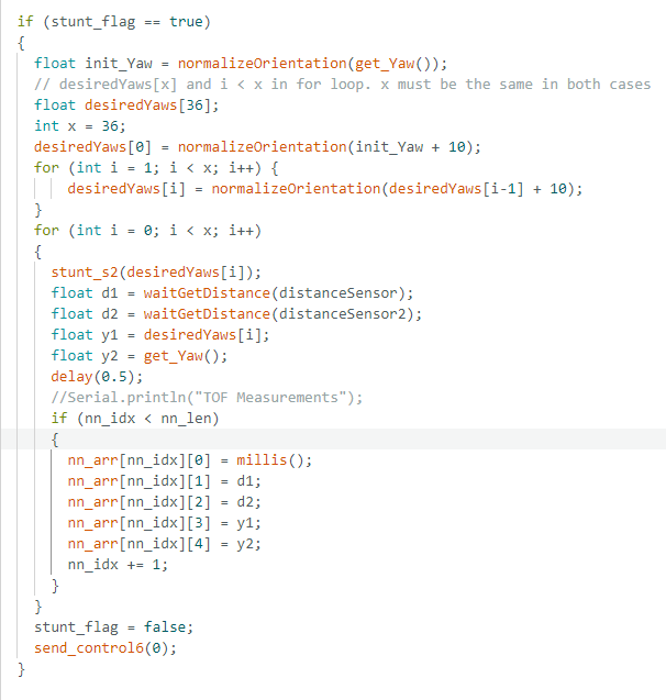
I then wrote the following code to turn my car 10 degrees 36 times.
I will explain the code below.
I first get the cars current DMP yaw position as detailed in earlier labs
from my function get_Yaw. I then create a float to store the desired Yaws
which stores 36 orientations of 10 degree increments. normalizeOrientation()
just keeps those values between [-180, 180].
After that my next loop calls stunt_s2 as detailed in a prior lab to do my
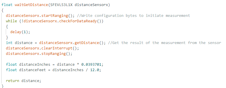
orientation control. When it reaches the desired orientation I call waitGetDistance()
which is a new method to wait until a ToF data point is received. Previously,
we had to implement a function to not wait for new data. I modified that function as shared
below to now wait until a measurement was received. Notice, I do collect data from both
ToF sensor measurements, leading to 72 possible points to interpret. I don't use a
Kalman Filter or interpolation as we want to only have sensor readings and not
predictions.
After that I get the desired Yaw and the real Yaw. I get both because I don't get the precise desired Yaw
since there is a threshold which it stops if anywhere within it.
After that, I added a small delay just for
safety even though the vehicle
was already stationary while awaiting ToF sensor values.
Then I save all four data points along with the timestamps in an array
to be sent back over bluetooth.
You can see a video of my PID controller working here along with the data
collected from the run:
Given my robot rotated around its axis within a 1 ft x 1ft square,
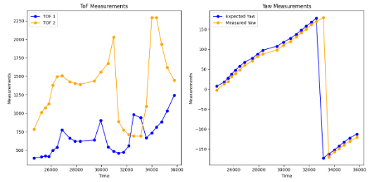
the offset would be up to 0.5 ft. Given my increments are 10 degrees,
the reason the above plot shows the measured to be consistently below the expected is because it stops as soon as
it is within 10 degrees, so on average it is anticipated to stop 10 degrees beneath the expected.
As a result, to evaluate its accuracy, since I'm using the measured yaw and not expected yaw, I estimate it based off of
it supposed to stop 10 degrees beneath the expected.
Given this, I found the maximum error to be 5 degrees on average for the error to be less than 2 degrees.
Furthermore, since I'm using a DMP, it handles the drift on its own so that is of minimal concern.
As a result, given all these factors, I would assume that given an accurate ToF sensor that my error
spinning in the middle of a 4x4 empty room
would be roughly
at maximum 0.7 ft off the true target and on average within 0.3 feet.
However, factoring in inaccuracy in the sensors would mean that I expect as the measurements, to get further
away, that the error would increase.
Processing Data
I share the polar plots as well as the 4 received data points for each of the four required points: (-3, -2), (5, 3), (0, 3), and (5, -3).
I started the vehicles in the same orientation pointing in the positive x-direction.
Plots of Data
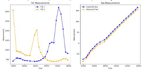
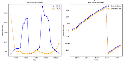
Below I share for all 4 points two charts. The first plot is 2 ToF plot measurements.
There will be large variations in the data for 4 main factors.
1) ToF sensors are placed on opposite sides of the car. So they are capturing different data.
Hence, the expected measurement lines up with the measurement captured 18 points later.
This is handled to make sure measurements line up with their expected orientation.
2) ToF sensors have different offsets from center of the car. These offsets are handled later.
3) ToF sensors will have noise and may vary depending on accuracy / precision. Hence, outliers are
removed later during mapping.
4) While turning the vehicle, the rotation on its axis is not 100% precise leading to slight variations in
expected measurement. This means one must assume a level of noise which is handled by removing variables that
are outliers and experiments to see if there is large variation between the two points that
are theoretically at the same angle after accounting for the above 3 possibilities.
The second plot is a comparison of the Expected Yaw to the Measured Yaw.Note, the raw data is shared below with no cleanups for the points made above.
In addition, I noticed after postprocessing that my arrays were dropping the datapoints at the end
since it filled the array at 25 points as opposed to 36 since I forgot to update it.
Unfortunately, due to lab hours I wasn't able to go back and collect all 36 points but since
I was using both sensors, I still managed to have enough data to get a 360 view of the entire map.
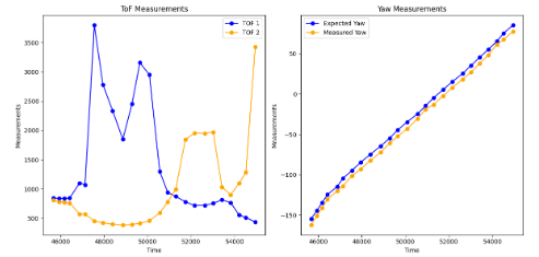
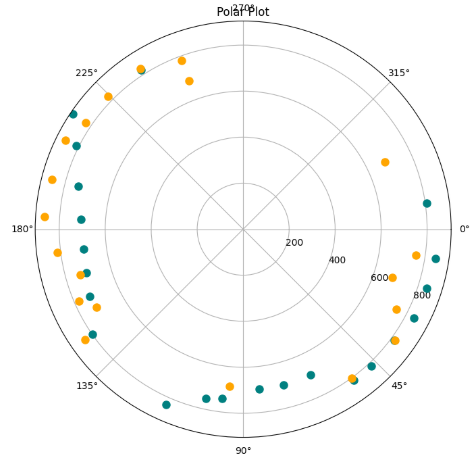
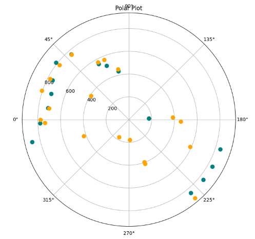
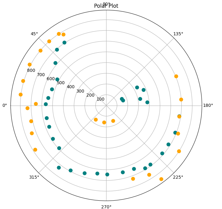
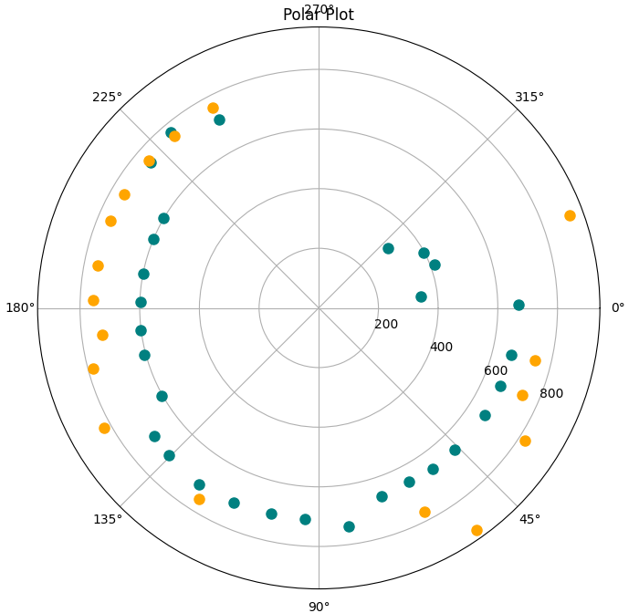
(5, -3)
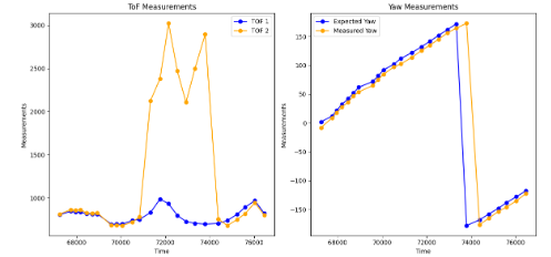
(5, 3)
(-3, -2)
(0, 3)
I decided to go with my DMP measured angles since the plots showed the DMP generally was in agreement
with my Expected Values.
Given that I built in a threshold for stopping, I determined that the DMP would more accurately
determine where in that threshold I was located and would help me plot more accurately what
angle I was at. This is because the precision of using my expected value would only be as good
as my given threshold.
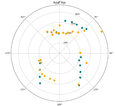
Polar Plots
For all the polar plots, the Teal represents measurements
from the first ToF and the orange represents measurements from the second
ToF. In addition, to prevent large outliers only points between
0.5-3 feet away were kept for the polar plots. Given that 50 (of the desired 72) points were recorded, noise
was bound to happen and some datapoints were ridiculously off and causing poor scale issues.
Keeping all measurements 0.5-3 feet away allowed to get the relevant points and enough points to
generalize about the walls without having the map be filled with
noise that was difficult to interpret. These points are shared below.
(5, -3)
(5, 3)
(-3, -2)
(0, 3)
I found these measurements to be reasonable, with the first 3 looking very clear
and the 4th being a little noisier but the wall shape could still be determined.
Even though after the data was cleaned with the basic checks I described above, there was still
noise, the general shape of the walls were observable and relatively accurate.
Then to check the precision of my scans I did two more rotations on the same point.
Below I share the results for the point (-3, -2) for 3 scans.
As one can observe, while the measurements are not precisely the same,
the rotations do all get the same relative shape that can be interpretted.
This demonstrates, that mapping can be done relatively accurately.
Merge and Plot Your Readings
Describe the Matrices and Plot All Your TOF sensor readings
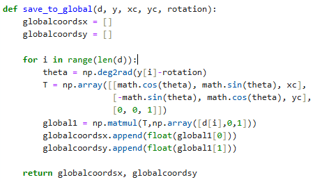
Initially, I had a ton of issues with plotting because in my rotation matrix
I set the - value to the wrong math.sin(theta) value. This led my values to be flipped
no matter the given rotation. Identifying this as a key issue I finally solved for it
and created a function save_to_global that would take in my distance measurement, my measured
yaw, and my x / y coordinates. In addition, I added a parameter rotation to allow
for adjustments so I could rotate the data as appropriate on the map.
The code is shared below.
One can see in my function that I get theta based
on the orientation of my points and then use it in my rotation
matrix T which has the vehicle's points (xc,yc). Then I multiply,
T by a 3x1 vector which is [ToF measurement, 0, 1].
These values are then output as the global coordinates in two
lists.
To prepare the data to go in, I processed all the data so that for all
values measured with my second time of flight sensor, was associated
with the opposite orientation. This was as simple as just taking the
data "d" and doing: d[:halfway_point] + d[halfwaypoint:]
In addition, I converted all the measured data into feet from mm
by multiplying by .00328084 so that the x and y coords I passed
into save_to_global would be accurate.
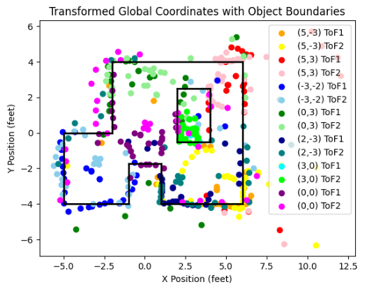
After all of that was complete, then I just plotted the new
global points that were output by my save_to_global function.
The result of that just filtering out data
that was detected at more than 10 feet away (since that is roughly
the width of the entire map)
is shared below. In addition, I include the line estimates of my map
and measured 3 additional points to the required four. These are
(2,-3), (3,0), (0,0).
While the first map had almost all the points shared.
This second plot, I filter out a lot of the points
and only keep points between 1 to 3 feet away. This provides
a cleaner picture of my estimates albeit with less points. As one can see
several walls are accurately mapped although there some obvious wrong
points, specifically in the below plot the purple points and some yellow points, that are
likely from the ToF sensor pointing somewhat at the ground.
I share my estimated lists for walls here:start = [(-2,4),(-5,-4),(-5,0),(1,-4),(-5,0),(-2,0),(6,4),(-1,-1.75),(1,-1.75),(-1,-4),(2,-.5),(2,2.5),(4,2.5),(4,-.5)]endit = [(6,4),(-1,-4),(-5,-4),(6,-4),(-2,0),(-2,4),(6,-4),(1,-1.75),(1,-4),(-1,-1.75),(2,2.5),(4,2.5),(4,-.5),(2,-.5)]